https://www.computer.org/csdl/journal/tp/2022/08/09361303/1rsezbEXNxS
Introduction 現在のPU Learningの多くはBiasを考慮せずに、Select Completely At Random(SCAR)の問題設定である。この論文では、Select At Random(SAR)のうち、Ground Truthのラベル y y y に依存せず、インスタンス x \mathbf{x} x にのみラベル付けされるかどうかの変数 s s s が依存する設定を考えている 。
つまり、PU Learningについて、SCARではP r ( s = 1 ∣ y = 1 , x ) = P r ( s = 1 ∣ y = 1 ) = η Pr(s=1|y=1,\mathbf{x}) = Pr(s=1|y=1)=\eta P r ( s = 1∣ y = 1 , x ) = P r ( s = 1∣ y = 1 ) = η P r ( s = 1 ∣ y = 1 , x ) = η ( x ) Pr(s=1|y=1,\mathbf{x}) = \eta(\mathbf{x}) P r ( s = 1∣ y = 1 , x ) = η ( x )
この論文では、確率的なアプローチであるLabeling Bias Estimation(LBE)について提案した。今の問題設定では、η ( x ) \eta(\mathbf{x}) η ( x ) P r ( y = 1 ∣ x ) , P ( x ) Pr(y=1|\mathbf{x}), P(\mathbf{x}) P r ( y = 1∣ x ) , P ( x )
これらについて、線形識別器とDNNの両方のモデルでそれぞれ実装する提案を行った。
提案手法はSingle-Training-Set(1set)の設定である。Case-Controlでは以下の「順序不変性」が成り立つ必要があるが強すぎる仮定ではないか、とこの論文は考えた。
順序不変性とは、ここではラベルがつきやすいければつきやすいほど、Positiveである。その逆も成り立つという仮定。 📄 2019-ICLR-[PUSB]Learning from Positive and Unlabeled Data with a Selection Bias
P r ( s = 1 ∣ y = 1 , x 1 ) ≤ P r ( s = 1 ∣ y = 1 , x 2 ) ⇔ P r ( y = 1 ∣ x 1 ) ≤ P r ( y = 1 ∣ x 2 ) Pr(s=1|y=1,\mathbf{x}_1) \leq Pr(s=1|y=1,\mathbf{x}_2) \\
\Leftrightarrow
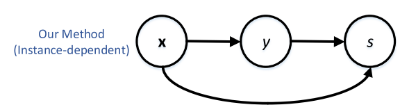
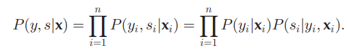
Pr(y=1|\mathbf{x}_1) \leq Pr(y=1|\mathbf{x}_2) P r ( s = 1∣ y = 1 , x 1 ) ≤ P r ( s = 1∣ y = 1 , x 2 ) ⇔ P r ( y = 1∣ x 1 ) ≤ P r ( y = 1∣ x 2 ) Proposed Method 問題設定 データは( x , y , s ) (\mathbf{x}, y, s) ( x , y , s ) データ本体はx ∈ X ⊆ R d \mathbf{x} \in X \subseteq \mathbb{R}^d x ∈ X ⊆ R d Ground Truthのラベルはy = 0 y=0 y = 0 y = 1 y=1 y = 1 s = 1 s=1 s = 1 s = 0 s=0 s = 0 全体的なグラフィカルモデル インスタンス依存なので、以下のようになる。
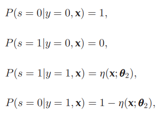
詳細な確率は以下の通り。
(1, 2行目)Ground TruthがNegativeの例に対して、ラベルは必ず付かない。(PUの問題設定) (3, 4行目)Ground TruthがPositiveの例に対して、ラベルがつく確率はPropensity Scoreのη ( x ; θ 2 ) \eta(\mathbf{x};\theta_2) η ( x ; θ 2 ) θ 2 \theta_2 θ 2 モデル化 それぞれ、以下のものを頑張ってモデル化してみる。
h ( x ; θ 1 ) = P r ( y = 1 ∣ x ) η ( x ; θ 2 ) = P r ( s = 1 ∣ y = 1 , x ) h(\mathbf{x};\theta_1) = Pr(y=1|\mathbf{x}) \\
\eta(\mathbf{x};\theta_2) = Pr(s=1|y=1, \mathbf{x}) h ( x ; θ 1 ) = P r ( y = 1∣ x ) η ( x ; θ 2 ) = P r ( s = 1∣ y = 1 , x ) これをロジスティックモデルでやったり( 1 + exp ( − θ 1 T x ) ) − 1 (1+\exp(-\theta_1 ^ T \mathbf{x}))^{-1} ( 1 + exp ( − θ 1 T x ) ) − 1
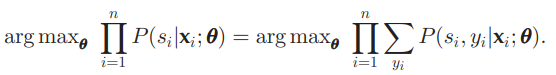
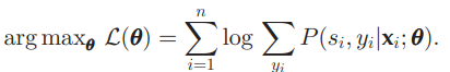
パラメタの学習 ここでのθ \theta θ θ 1 , θ 2 \theta_1, \theta_2 θ 1 , θ 2
右辺について、logをとって最小化するのを考える。
ここで、隠れ変数を y i y_i y i とすることで、 P ( y i ∣ s i , x i ) P(y_i | s_i, \mathbf{x}_i) P ( y i ∣ s i , x i ) のモデルがわかっている前提で log P ( s i ∣ x i ; θ ) \log P(s_i | \mathbf{x}_i; \theta) log P ( s i ∣ x i ; θ ) をEM Algorithmで推定できる。
📄 EM Algorithmの解説
具体的には、以下のようなELBOの最大化を考える。
log P ( s i ∣ x i ; θ ) = E L B O + D K L ( q ( y i ) ∣ ∣ p ( y i ∣ s i , x ) ) E L B O = E q ( y i ) [ log p ( x , s i , y i ) − log q ( y i ∣ s i , x ) ] = E q ( y i ∣ s i , x ) [ log p ( s i , x ∣ y i ) ] + E q ( y i ∣ s i , x ) [ log p ( y i ) − log q ( y i ∣ s i , x ) ] \log P(s_i | \mathbf{x}_i;\theta) = ELBO + D_{KL}(q(y_i)||p(y_i|s_i, \mathbf{x})) \\
ELBO = \mathbb{E}_{q(y_i)} [\log p(\mathbf{x}, s_i, y_i) - \log q(y_i|s_i, \mathbf{x})] \\
= \mathbb{E}_{q(y_i|s_i, \mathbf{x})} [\log p(s_i, \mathbf{x}|y_i)] + \mathbb{E}_{q(y_i|s_i, \mathbf{x})} [\log p(y_i) - \log q(y_i|s_i, \mathbf{x})] log P ( s i ∣ x i ; θ ) = E L BO + D K L ( q ( y i ) ∣∣ p ( y i ∣ s i , x )) E L BO = E q ( y i ) [ log p ( x , s i , y i ) − log q ( y i ∣ s i , x )] = E q ( y i ∣ s i , x ) [ log p ( s i , x ∣ y i )] + E q ( y i ∣ s i , x ) [ log p ( y i ) − log q ( y i ∣ s i , x )] Eステップ ここでは、ELBOの最大化のために、q q q q ( y i ) = p ( y i ∣ s i , x ) q(y_i) = p(y_i | s_i, \mathbf{x}) q ( y i ) = p ( y i ∣ s i , x )
ここで、以下のようにp ( y i ∣ s i , x i ) p(y_i | s_i, \mathbf{x}_i) p ( y i ∣ s i , x i )
ここで、 P ( y i ∣ x i , s i ) = P ( s i , y i ∣ x i ) / P ( s i ∣ x i ) P(y_i|\mathbf{x}_i, s_i) = P(s_i, y_i|\mathbf{x}_i)/P(s_i|\mathbf{x}_i) P ( y i ∣ x i , s i ) = P ( s i , y i ∣ x i ) / P ( s i ∣ x i ) であり、分母は明らかに y i y_i y i の関数ではなく、定数なので q ( y i ) q(y_i) q ( y i ) の最適化に不要だから。
Mステップ 次に、q q q p ( y i ∣ s i , x i ) p(y_i|s_i, \mathbf{x}_i) p ( y i ∣ s i , x i )
これは、以下の式を最大化する。
arg max θ ∑ y i p ( y i ∣ x i , s i , θ o l d ) log p ( x i , s i , y i ∣ θ ) = 𝔼 y i ∣ s i , x i , θ o l d [ log p ( x i , s i , y i ∣ θ ) ] \argmax_\theta \sum_{y_i} p(y_i|\mathbf{x}_i, s_i, \theta _{old}) \log p(\mathbf{x}_i, s_i, y_i|θ) = 𝔼 _{y_i|s_i, \mathbf{x}_i, \theta _{old}}[\log p(\mathbf{x}_i, s_i, y_i|θ)] arg max θ ∑ y i p ( y i ∣ x i , s i , θ o l d ) log p ( x i , s i , y i ∣ θ ) = E y i ∣ s i , x i , θ o l d [ log p ( x i , s i , y i ∣ θ )] ここで、p ( x i , s i , y i ∣ θ ) p(\mathbf{x}_i, s_i, y_i | \theta) p ( x i , s i , y i ∣ θ )
log p ( x i , s i , y i ∣ θ ) = log p ( x i ∣ θ ) + log p ( s i ∣ x i , θ ) + log p ( y i ∣ x i , s i , θ ) \log p(\mathbf{x}_i, s_i, y_i | \theta) = \log p(\mathbf{x}_i | \theta) + \log p(s_i|\mathbf{x}_i, \theta) + \log p(y_i | \mathbf{x}_i, s_i, \theta) log p ( x i , s i , y i ∣ θ ) = log p ( x i ∣ θ ) + log p ( s i ∣ x i , θ ) + log p ( y i ∣ x i , s i , θ ) ここで、第一項の p ( x i ∣ θ ) p(\mathbf{x}_i | \theta) p ( x i ∣ θ ) は、パラメタによって p ( x i ) p(\mathbf{x}_i) p ( x i ) を近似しているといえるが、これは既知というか定数であると考える(データの分布は変わらない)なら、最大化するのは2つの項のみである。
EMアルゴリズムはこうやってわかっている部分をどんどん削ぎ落していい。
残った2つの項について、h , η h, \eta h , η を用いて対数尤度 を計算できるので、これでOKである。
最後に、これの最大化はGradient Ascend によって行う。
Noisy Label PUデータへの対処 h ( x ; θ 1 ) = P r ( y = 1 ∣ x ) h(\mathbf{x};\theta_1) = Pr(y=1|\mathbf{x}) h ( x ; θ 1 ) = P r ( y = 1∣ x ) h 2 ( x ; θ 2 ) h_2(\mathbf{x};\theta_2) h 2 ( x ; θ 2 )
h ( x ; θ 1 ) ⋅ h 2 ( x ; θ 2 ) h(\mathbf{x};\theta_1) \cdot h_2(\mathbf{x};\theta_2) h ( x ; θ 1 ) ⋅ h 2 ( x ; θ 2 ) このように信頼度を乗じた重み付きの学習とすることで対処するらしい。
この論文では、 h 2 h_2 h 2 は同様に確率的にモデル化されている。これも同様にロジスティック回帰や多層パーセプトロンらしい。
Eステップの時に、p ( y i ∣ x i , s i ) p(y_i|\mathbf{x}_i, s_i) p ( y i ∣ x i , s i ) q ( y i ) q(y_i) q ( y i ) p ( y i = 1 ∣ x i , s i ) p(y_i=1|\mathbf{x}_i, s_i) p ( y i = 1∣ x i , s i ) h 2 ( x i ; θ 2 ) h_2(\mathbf{x}_i;\theta_2) h 2 ( x i ; θ 2 ) 普通にMステップでθ 2 \theta_2 θ 2 これ系でいつものことだが、Warm upは当然必要だろうしNoisy Rateが高いと辛そう。
あと2つも θ 1 , θ 2 \theta_1, \theta_2 θ 1 , θ 2 とパラメタ更新が必要なモデルがあると学習不安定になりそう。
Experiments Baselineの手法は以下のようなもの。📄 2015-ICML-[uPU] Convex Formulation for Learning from Positive and Unlabeled Data 📄 2017-NIPS-[nnPU] Positive-Unlabeled Learning with Non-Negative Risk Estimator [LDCE] C. Gong, H. Shi, T. Liu, C. Zhang, J. Yang, and D. Tao, “Loss decomposition and centroid estimation for positive and unlabeled learning,” IEEE Trans. Pattern Anal. Mach. Intell., vol. 43, no. 3, pp. 918–932, Mar. 2021 📄 2019-ECML PKDD-[PWE]Beyond the Selected Completely At Random Assumption for Learning from Positive and Unlabeled Data データセットはガウス分布による合成データセットと、実データセット。テーブルデータのような次元数が低いデータセットは、australian, madelon, phishing, vote, banknote, breastを使った。 実データセットはUSPS、HockeyFight、SwissProtを使用。USPSは手書き数字。 HockeyFightはアイスホッケーでの暴力行為の検出らしい。結構難しいデータセット。 SwissProtは、文書分類のPUのデータセット。バイアスを含んでいてバイアスあるPUの手法のテストによく使われる。 バイアスについては以下のように選択する。κ \kappa κ 決定境界から遠いPほどラベル付けされやすい。ラベルがつくかどうかの関数h ( x ) h(\mathbf{x}) h ( x ) h ( x ) = ( 1 1 + exp ( − θ T x ) ) κ h(\mathbf{x}) = (\frac{1}{1 + \exp(-\theta ^ T \mathbf{x})})^\kappa h ( x ) = ( 1 + e x p ( − θ T x ) 1 ) κ 決定境界から近いPほどラベル付けされやすい。難しいサンプルほどラベルがつくという形。h ( x ) = ( 1 − 1 1 + exp ( − θ T x ) ) κ h(\mathbf{x}) = (1 - \frac{1}{1 + \exp(-\theta ^ T \mathbf{x})})^\kappa h ( x ) = ( 1 − 1 + e x p ( − θ T x ) 1 ) κ


 2015-ICML-[uPU] Convex Formulation for Learning from Positive and Unlabeled Data